![[David Silver] 5. Model-Free Control: On-policy (GLIE, SARSA), Off-policy (Importance Sampling, Q-Learning)](https://img1.daumcdn.net/thumb/R750x0/?scode=mtistory2&fname=https%3A%2F%2Fblog.kakaocdn.net%2Fdn%2Fc0t9Fe%2FbtryXfC0q7I%2Fz27IjenKvGuPor7Fk5zcpk%2Fimg.png)
이 글은 필자가 David Silver의 Reinforcement Learning 강좌를 듣고 정리한 글입니다.
In the previous post, to solve an unknown MDP we had to (1) Estimate the value function (Model-Free Prediction) and (2) Optimize the value function (Model-Free control). In this lecture, we are going to learn (2) how to optimize the value function based on the (1) methodologies which are MC and TD.
So the goal which we have to achieve is on policy iteration,
- Policy evaluation: So far there are MC and TD
- Policy improvement How are we going to integrate Greedy policy improvement based on those policy evaluation methodologies? The answer would be Monte-Carlo control or Temporal-Difference control.
🥁 On-policy vs. Off-policy
차이가 확실히 아직 느껴지지 않는다.
- On-policy learning: Learn about policy π from experience sampled from π
- Off-policy learning: Learn about policy π from experience sampled from μ
- Following behavior policy μ(a|s), {S1,A1,R2,⋯,ST}∼μ
- Why is this important?
- Learn about optimal policy while following exploratory policy
- Learn from observing humans or other agents
- Re-use experience generated from old policies π1,π2,⋯,πt−1
- Learn about multiple policies while following one policy
🥁 ϵ-Greedy policy improvement
- Before) Greedy Policy Improvement
- Greedy policy improvement over Q(s,a) is model free π′(s)=argmax
- No exploration
- After) \epsilon-Greedy Policy Improvement
- Simplest idea for ensuring continual exploration.
- All m are tried with non-zero probability.
- With probability 1-\epsilon choose the greedy action.
\pi (a|s) =
🥁 On-policy Monte-Carlo control: GLIE
Greedy in the Limit with Infinite Exploration (GLIE): If all station-action pairs are explored infinitely many times, the policy converges on a greedy policy.
For every episode:
- Policy evaluation Monte-Carlo policy evaluation, Q \approx q_\pi
- Sample kth episode using \pi: \big\{ S_1, A_1, R_2, \cdots , S_T \big\} \sim \pi
- For each state S_t and action A_t in the episode,
- N(S_t, A_t) \leftarrow N(S_t, A_t) + 1
- Q(S_t, A_t) \leftarrow Q(S_t, A_t) + \frac{1}{N(S_t, A_t)} (G_t - Q (S_t, A_t))
- Policy improvement \epsilon-greedy policy improvement
- Improve policy based on new action-value function
- \epsilon \leftarrow \frac{1}{k}, \pi \leftarrow \epsilon \textrm{-greedy}(Q)
- Improve policy based on new action-value function
🥁 On-policy Temporal-Difference control: SARSA
For every time-step
- Policy evaluation SARSA, Q \approx q_\pi
- Update action-value functions with SARSA Q(S, A) \leftarrow Q(S,A) + \alpha (R + \gamma Q(S', A')-Q(S,A))
- Policy improvement \epsilon-greedy policy improvement
🥁 Deeper in SARSA
- n-Step SARSA updates Q(s,a) towards the n-step Q-return Q(S_t, A_t) \leftarrow Q(S_t, A_t) + \alpha (q_t^{(n)}-Q(S_t, A_t))
- Forward view SARSA(\lambda) Q(S_t, A_t) \leftarrow Q(S_t, A_t) + \alpha (q_t^{\lambda}-Q(S_t, A_t))
- Backward view SARSA(\lambda) $Q(S_t, A_t) \leftarrow Q(S_t, A_t) + \alpha \delta_t E_t(s,a)$
- TD-error \delta_t = R_{t+1}+\gamma Q(S_{t+1}, A_{t+1}) - Q(S_t, A_t)
- Eligibility trace for each state-action pair E_t (s,a) = \gamma \lambda E_{t-1}(s,a) + 1(S_t=s, A_t=a)
- SARSA(\lambda)

🥁 Off-Policy Learning: Importance Sampling
- As we have a target policy \pi (a|s) and behavior policy \mu(a|s), we can estimate the return between policies (\pi, \mu) using importance sampling:
$ \mathbb{E}_{X \sim P} [f(X)] = \mathbb{E}_{X \sim Q} [\frac{P(X)}{Q(X)}f(X)]$
$\mathbb{E}_{X \sim P} [f(X)] = \mathbb{E}_{X \sim Q} [\frac{P(X)}{Q(X)}f(X)]$
🥁 Importance Sampling for Off-Policy Monte-Carlo
For compute the returns generated from \mu to evaluate \pi, we can multiply the importance sampling corrections along whole episode
$G^{\frac{\pi}{\mu}}_t = \frac{\pi(A_t|S_t)}{\mu(A_t|S_t)} \frac{\pi(A_{t+1}|S_{t+1})}{\mu(A_{t+1}|S_{t+1})} \cdots \frac{\pi(A_{T}|S_{T})}{\mu(A_{T}|S_{T})}G_t$
Update value towards corrected return
V(S_t) \leftarrow V(S_t) + \alpha (G_t^{\frac{\pi}{\mu}}-V(S_t))
But we cannot use this because (1) if \mu is zero when \pi is non-zero (2) Importance sampling can dramatically increase variance.
🥁 Importance Sampling for Off-Policy TD
We can use off-policy when we implement on TD. We only need a single importance sampling correction.
V(S_t) \leftarrow V(S_t) + \alpha (\frac{\pi (A_t|S_t)}{\mu (A_t|S_t)} (R_{t+1}+ \gamma V(S_{t+1}))-V(S_t))
Because policies only need to be similar over a single step, this has much lower variance than Monte-Carlo importance sampling.
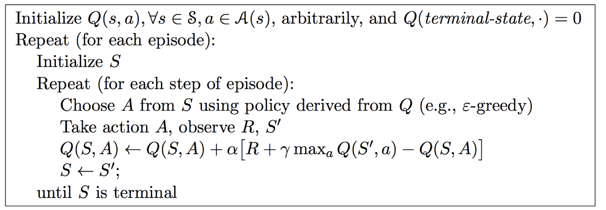
🥁 Off-Policy Control with Q-Learning
- On on-policy, next action is chosen using behavior policy A_{t+1} \sim \mu(. | S_t). But we consider alternative successor action A' \sim \pi (.|S_t) and update Q(S_t, A_t) towards value of alternative action
Q(S_t, A_t) \leftarrow Q(S_t,A_t) + \alpha (R_{t+1} + \gamma Q(S_{t+1}, A')-Q(S_t, A_t))
- So we can allow both behavior and target policies to improve
- The target policy \pi is greedy \pi(S_{t+1})= \arg \max_{a'} Q(S_{t+1}, a')
- The behavior policy \mu is \epsilon-greedy
- The Q-learning target then simplifies:
R_{t+1} + \gamma Q(S_{t+1}, A') = R_{t+1} + \gamma Q(S_{t+1}, \arg \max_{a'} Q(S_{t+1}, a')) = R_{t+1} + \max_{a'} \gamma Q(S_{t+1}, a')
- Q-Learning
🥁 Summarize SARSA

'Robotics & Perception > Reinforcement Learning' 카테고리의 다른 글
| [David Silver] 7. Policy Gradient: REINFORCE, Actor-Critic, NPG (0) | 2022.04.10 |
|---|---|
| [David Silver] 6. Value Function Approximation: Experiment Replay, Deep Q-Network (DQN) (0) | 2022.04.10 |
| [David Silver] 4. Model-Free Prediction: Monte-Carlo, Temporal-Difference (0) | 2022.04.09 |
| [David Silver] 3. Planning by Dynamic Programming (0) | 2022.04.02 |
| [David Silver] 2. Markov Decision Processes (0) | 2022.04.02 |