[David Silver] 4. Model-Free Prediction: Monte-Carlo, Temporal-Difference

 

 

이 글은 필자가 David Silver의 Reinforcement Learning 강좌를 듣고 정리한 글입니다.

The last lecture was about Planning by Dynamic Programming, which solves a known MDP. Now we are going to check how can we solve an unknown MDP (i.e. Model-free RL). To solve an unknown MDP we have to (1) Estimate the value function of an unknown MDP. We usually call this Model-free prediction(Policy evaluation). After that, we will (2) Optimize the value function of an unknown MDP which we call it Model-Free Control. In this lecture, we are going to learn about the Model-free Prediction methodology, which consists of Monte-Carlo and Temporal-Difference.

We have to focus on how Monte-Carlo and Temporal-Difference methodology estimate the value function $v_\pi$ of an unknown MDP(Then what consists of unknown MDP? How can we get the G_t? "No knowledge of MDP transitions/rewards").

• Goal: learn $v_\pi (=\mathbb{E}_\pi [G_t|S_t=s])$ from episodes of experience under policy $\pi$ 
  • $S_1, A_1, R_2, \cdots, S_k \sim \pi$

🌳 Monte-Carlo Policy Evaluation

• MC methods
  • learn directly from complete episodes of experience. On Monte-Policy Evaluation, it uses empirical mean return instead of expected return.
  • Caveat: can only apply MC to episodic MDPs
    • All episodes must terminate
• Monte-Carlo Policy Evaluation
  • To evaluate state $s$, they update state $s$ is visited in an episode from the first time-step or every time-step. (Temporal Difference = Incremental every-visit Monte-Carlo)
  • Plain Update: Value is estimated by mean return $V(s) =\frac{S(s)}{N(s)}$. By law of large numbers, $V(s) \rightarrow v_\pi(s)$ as $N(s) \rightarrow \infty$ 
    1. Increment counter $N(s) \leftarrow N(s) + 1$ 
    2. Increment total return $S(s) \leftarrow S(s) + G_t$
  • Incremental Monte-Carlo Updates: Update $V(s)$ incrementally after episode $S_1, A_1, R_2, \cdots, S_T$. For each state $S_t$ with return $G_t$
    1. Increment counter $N(S_t) \leftarrow N(S_t) + 1$
    2. Increment total return $V(S_t) \leftarrow V(S_t) + \frac{1}{N(S_t)} (G_t-V(S_t))$. (If non-stationary problem, it can be useful to track a running mean, i.e. forget old episodes: $V(S_t) \leftarrow V(S_t) + \alpha (G_t-V(S_t))$
  • MC converges to solution with minimum mean-squared error

🌳 Temporal-Difference Policy evaluation

• TD methods
  
  • TD learns directly from incomplete episodes, by bootstrapping. learn $v_\pi$ online from experience under policy $\pi$. 
• Temporal-Difference Policy Evaluation
  • To evaluate state $s$, they update state $s$ is visited in an episode from every time-step: Incremental every-visit Monte-Carlo.
  • How to Update: Update $V(S_t)$ toward estimated reward $R_{t+1} + \gamma V(S_{t+1})$: $V(S_t) \longleftarrow V(S_t) + \alpha (R_{t+1} + \gamma V(S_{t+1})-V(S_t))$ 
    • TD error: $\delta=R_{t+1}+\gamma V(S_{t+1})-V(S_t)$ 
    • TD target: $R_{t+1}+\gamma V(S_{t+1})$ 
      • TD target is biased estimate of $v_\pi (S_t)$. 
      • True (Unbiased) TD target is $R_{t+1}+\gamma v_\pi (S_{t+1})$
      • Unbiased estimate (pi?전체 episode에 대한 정보를 바탕으로 Update 해야 하는데 한 스텝에서만의 대한 처리라서 그런가? 근데 왜 policy가 여기서 나오지? episode 아닌가?. TD(0) converges to $v_\pi(s)$는 무슨 뜻인가.$)of $v_\pi (S_t)$ is Return: $G_t = R_{t+1}+\gamma R_{t+2}+\cdots +\gamma^{T-1}R_T$
      • TD target is much lower variance than the return. Because return depends on many random actions, transitions, rewards. TD target depends on one random action, transition, reward.
  • TD(0) converges to solution of max likelihood Markov model

🌳 MC vs. TD

Temporal-Difference	Monte-Carlo
learn before knowing the final outcome (online learning)	wait until end of episode before return is known.
$V(S_t) \leftarrow V(S_t) + \alpha (R_{t+1}+\gamma V(S_{t+1})-V(S_t))$	$V(S_t) \leftarrow V(S_t) + \alpha (G_t-V(S_t))$
learn without the final outcome / works in continuing (non-terminating) environments.	only works for episodic (terminating) environments.
Low variance, Some bias	High variance, Zero bias
Usually more efficient than MC	Good convergence properties
More sensitive to initial value	Not very sensitive to initial value
Exploits Markov property / Usually more efficient in Markov environment	Do not exploit Markov property / Usually more effective in non-Markov environments.
Bootstraps	No bootstrap
Samples	Samples

• Dynamic Programming $V(S_t) \leftarrow \mathbb{E}_\pi [R_{t+1}+\gamma V(S_{t+1})]$
  • Bootstraps, No sample
• Unified View of Reinforcement Learning

David Silver's Lecture 4. Unified View of Reinforcement Learning

🌳 Deeper on Temporal-Difference 

• n-step TD
  • n-step return $G_t^{(n)}=R_{t+1}+\gamma R_{t+2}+\cdots \gamma^{n-1}R_{t+n}+\gamma^nV(S_{t+n})$
  • The $\lambda$-return $G_t^\lambda$ combines all n-step returns $G_t^{(n)}$ using decay $\lambda$: $G_t^\lambda =(1-\lambda)\sum_{n=1}^\infty \lambda^{n-1}G_t^{(n)}$
  • n-step TD learning $V(S_t) \leftarrow V(S_t) + \alpha (G_t^{(n)}-V(S_t))$
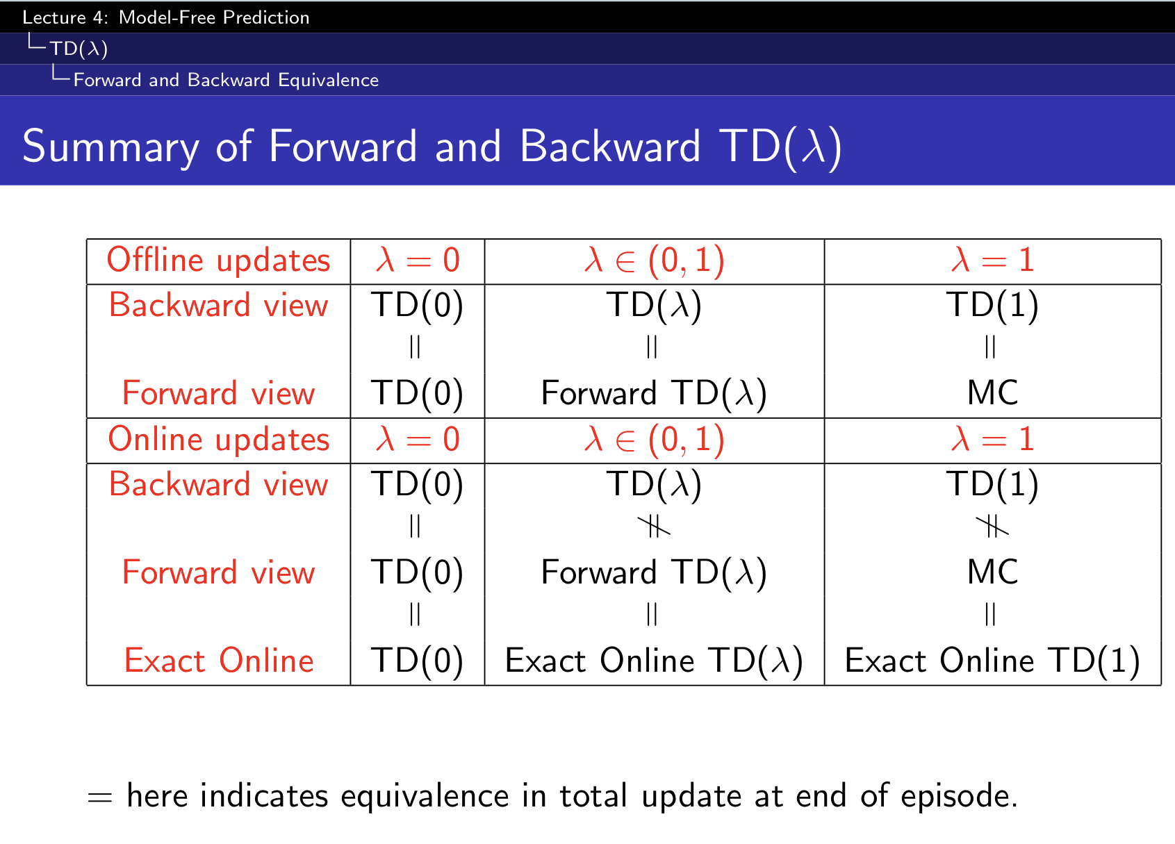
• Forward view of TD($\lambda$) $V(S_t) \leftarrow V(S_t) + \lambda (G_t^{\lambda}-V(S_t))$
  • Update value function $V(s)$ towards the $\lambda$-return
  • Foward-view looks into the future to compute $G_t^\lambda$
    • if $\lambda = 0$, only current state is updated
    • when $\lambda=1$, credit is deferred until end of episodes (Equivalent to every-visit Monte-Carlo)
  • Like MC, can only be computed from complete episodes
• Backward view of TD($\lambda$) $V(s) \leftarrow V(s) + \alpha \delta_t E_t(s)$  (TD-error $\delat_t$)
  • Update value function $V(s)$ for online, every step $s$, from incomplete sequence
  • Keep an eligibility trace for every state $s$
    • Frequency heuristic: assign credit to most frequent states
    • Recency heuristic: assign credit to most recent states
• Sum

Summary of Forward and Backward TD($\lambda$)